Deploying Diverse Regression Machine Learning Algorithms: An Implementation Overview

In this current post, we go into the exploration and analysis of various regression machine learning methods. Our objective is to utilize a range of machine learning techniques to forecast the load demand of the Cyprus power system.

In the initial phase, the ‘data’ dataframe include all essential features and measurements spanning a 16-month period. Throughout the analysis, our focus is directed towards two important features: temperature and hour. While incorporating additional features could potentially enhance result accuracy, for code explanation and methodology simplification, we have opted to retain only these two key features.

import matplotlib.pyplot as plt
import numpy as np

# Create a scatter plot with demand as color
plt.scatter(data['hour'], data['T2M'], c=data['Demand'], cmap='plasma', s=50)

# Add colorbar
cbar = plt.colorbar()
cbar.set_label('Demand (MW)')

# Set labels for axes
plt.xlabel('Hour of the Day')
plt.ylabel('Temperature (°C)')

plt.title('Temperature vs Hour (Color-coded by Demand)')

plt.show()

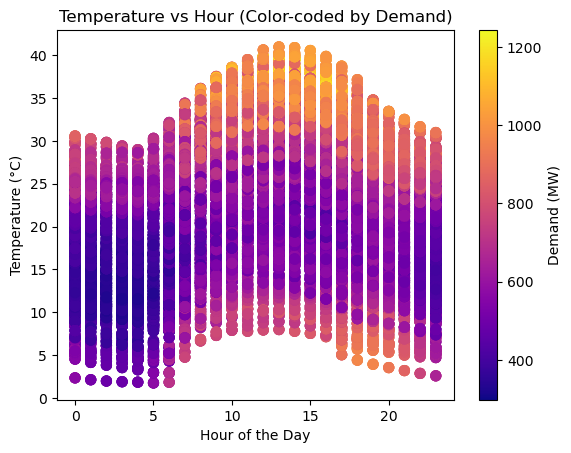
The first analysis illustrates the fluctuation of demand in megawatts (MW) in response to variations in temperature and hour. In instances of low demand, the figure showcases a darker color, transitioning to brighter hues as demand increases.

Data’s preparation

Prior to normalizing the data, it’s crucial to recognize that the ‘hour’ feature is cyclical. A detailed analysis on handling cyclical features has been discussed in a previous post, accessible here. Furthermore, the guidance on scaling data developed in other post here, Normalisation and Standardisation method implemented. Moreover, the data’s was divided into test and training data.

from sklearn.preprocessing import StandardScaler
sc=StandardScaler()
data.loc[:,['hour_sin','hour_cos','T2M_norm']]=sc.fit_transform(data.loc[:,['hour_sin','hour_cos','T2M']])

from sklearn.model_selection import train_test_split
X_train, X_test, y_train, y_test = train_test_split(X, y, test_size = 0.2, random_state = 0)

Assessing Machine Learning Regression Models: RMSE and R-squared Evaluation

When it comes to checking how well a machine learning regression model is doing, we use two important measures: RMSE and R-squared. RMSE looks at the average difference between the predicted values and the actual values. If the RMSE is low, it means the model is doing a good job. R-squared, on the other hand, tells us how much of the variability in the data our model can explain. A higher R-squared is better, showing that the model fits the data well. So, by looking at both RMSE and R-squared, we can figure out if our regression model is accurate and how well it explains the data.

from sklearn.metrics import r2_score
from sklearn.metrics import mean_squared_error
# Calculate RMSE
rmse = np.sqrt(mean_squared_error(y_test, X_test[:,5]))

# Calculate R-squared
r_squared = r2_score(y_test, X_test[:,5])

print(f'RMSE: {rmse}')
print("R-squared:", r_squared)

Current TSO’s demand forecast accuracy: RMSE= 30.194821557544707 , R-squared= 0.9700502334373836

1. Multiple Linear Regression

Multiple Linear Regression is a statistical technique that helps us make predictions by analyzing the relationships between multiple variables. Imagine you have a dataset with one outcome you want to predict (let’s call it ‘Y’) and several factors that might influence it (let’s call them ‘X1,’ ‘X2,’ etc.).

$\begin{center} Multiple Linear Regression: \[ Y = b_0 + b_1X_1 + b_2X_2 + \ldots + b_kX_k \] \end{center}$

The goal is to find the best values for b0,b1,…,bk that minimize the difference between our predicted Y and the actual Y in our dataset. Once we find these values, we can use them to make predictions. For example, if we want to predict someone’s weight (Y), we’d use their height (X1), age (X2), and other relevant factors. The coefficients (b0,b1,…,bk) tell us how much Y is expected to change for a one-unit change in each X variable, holding other variables constant. A positive coefficient means an increase in Y with an increase in the corresponding X, and a negative coefficient means the opposite.

Implementation of Multiple Linear Regression

# Training the Simple Linear Regression model on the Training set
from sklearn.linear_model import LinearRegression
MLR = LinearRegression()
MLR.fit(X_train[:,:3], y_train)

# Predicting the Test set results
y_predMLR = MLR.predict(X_test[:,:3])

from sklearn.metrics import r2_score
from sklearn.metrics import mean_squared_error
# Calculate RMSE
rmse = np.sqrt(mean_squared_error(y_test, y_predMLR))

# Calculate R-squared
r_squared = r2_score(y_test, y_predMLR)

print(f'RMSE: {rmse}')
print("R-squared:", r_squared)

2. Polyonimial Regression

Polynomial regression focuses on capturing nonlinear patterns by introducing higher-degree polynomial terms of a single independent variable. Polynomial regression is particularly useful when the relationship between the variables is nonlinear, providing a more accurate fit to the data compared to the linear assumptions of multiple linear regression.

$\begin{center} Polynomial Regression: \[ Y = b_0 + b_1X + b_2X^2 + \ldots + b_nX^n \] \end{center}$

Implementation of Polyonimial Regression

from sklearn.preprocessing import PolynomialFeatures
from sklearn.linear_model import LinearRegression
from sklearn.pipeline import make_pipeline

# Assuming X_train is your feature matrix with 3 columns, and y_train is your target variable

# Create a polynomial regression model with degree 2 (you can change the degree as needed)
degree = 2
PR = make_pipeline(PolynomialFeatures(degree), LinearRegression())

# Train the model
PR.fit(X_train[:,:3], y_train)

# Make predictions
y_predPR = PR.predict(X_test[:,:3])

from sklearn.metrics import mean_squared_error
# Calculate RMSE
rmse = np.sqrt(mean_squared_error(y_test, y_predPR))

# Calculate R-squared
r_squared = r2_score(y_test, y_predPR)

print(f'RMSE: {rmse}')
print("R-squared:", r_squared)

Implementation Support Vector Regression

# Training the SVR model on the whole dataset
from sklearn.svm import SVR
SVR = SVR(kernel = 'rbf')
SVR.fit(X_train[:,:3], y_train)

# Predicting a new result
y_predSVR=SVR.predict(X_test[:,:3])

print(np.concatenate((y_predSVR.reshape(len(y_predSVR),1), y_test.reshape(len(y_test),1)),1))
from sklearn.metrics import mean_squared_error
# Calculate RMSE
rmse = np.sqrt(mean_squared_error(y_test, y_predSVR))
# Calculate R-squared
r_squared = r2_score(y_test, y_predSVR)

print(f'RMSE: {rmse}')
print("R-squared:", r_squared)

Implementation Disicion Tree Regression

# Training the Decision Tree Regression model on the whole dataset
from sklearn.tree import DecisionTreeRegressor
DTR = DecisionTreeRegressor(random_state = 0)
DTR.fit(X_train[:,:3], y_train)
# Predicting a new result
y_predDTR=DTR.predict(X_test[:,:3])
from sklearn.metrics import mean_squared_error
# Calculate RMSE
rmse = np.sqrt(mean_squared_error(y_test, y_predDTR))
# Calculate R-squared
r_squared = r2_score(y_test, y_predDTR)
print(f'RMSE: {rmse}')
print("R-squared:", r_squared)

Implementation Random Forest Regression

# Training the Random Forest Regression model on the whole dataset
from sklearn.ensemble import RandomForestRegressor
RFR = RandomForestRegressor(n_estimators = 10, random_state = 0)
RFR.fit(X_train[:,:3], y_train)
# Predicting a new result
y_predRFR=RFR.predict(X_test[:,:3])
from sklearn.metrics import mean_squared_error
# Calculate RMSE
rmse = np.sqrt(mean_squared_error(y_test, y_predRFR))
# Calculate R-squared
r_squared = r2_score(y_test, y_predRFR)
print(f'RMSE: {rmse}')
print("R-squared:", r_squared)

Results

	TSO’s Forecast	Multiple Linear Regression	Polyonimial Regression	Support Vector Regression	Disicion Tree Regression	Random Forest Regression
RMSE	30.2	109.9	63.1	59.7	27.3	29.4
R-Squared	0.970	0.603	0.869	0.883	0.976	0.972

Your thoughts and questions are important for me. Feel free to share your insights or inquire about anything in the comments section below. Let’s keep the conversation going!

Leave a Comment Cancel Reply